Accelerating machining processes

The MC-SUITE project proposes a new generation of ICT enabled process simulation and optimization tools enhanced by physical measurements and monitoring that can increase the competence of the European manufacturing industry, reducing the gap between the programmed process and the real part.

Automatization of the full machining process using ProActive workflows

Figure 1: The full machining process

The workflow controls the complete execution of all tools involved in the virtual machining process and automatically manages file transfers between tool executions. Figure 1 depicts the graphical representation of the orchestration xml file.Using dataspaces is crucial since tasks are submitted to ProActive nodes that could live remotely. Therefore, required files by a task must be placed in the scheduler dataspace to be automatically transferred to the running task temporary dir. To achieve that, ProActive provides dedicated tags (transferFromUserSpace, transferToUserSpace,...). Moreover, files will be referred from the task script using the file name, i.e. without specifying the path.

This workflow suffers from a lack of automatization. Indeed, the CAD task pops up a GUI, requiring parameters to be set for the Himill configuration file generation. This step breaks the full procedure automatization. To tackle that, we proposed an updated version of the workflow by first, migrating all the CAD parameters in the workflow parameters section. This can be easily achieved since the orchestration code follows the xml syntax, clearly separated from the functional code.
 removing the CAD task and the CAD installation path parameter. Then by adding a groovy section to dynamically generate the Himill configuration file according to the workflows parameters. Each task supports most of the main programming language, and we used Groovy which offers advanced methods to easily work with .ini files.

A study of the the parallel stability lobes research using Matlab/Scilab ProActive connectors

 Matlab is the most productive software environment for engineers and scientists. Matlab is widely used in many industrial and research projects. Using connectors from the Matlab GUI, you can execute in parallel Matlab functions, use blocking commands to wait for all tasks results or one of them, create your own workflow of computational functions directly from your Matlab GUI, manage file transfer, start a fault-tolerant session,...

 >res = PAsolve (@factorial, 1, 2, 3, 4, 5)
 Job submitted : 2
Awaited (J:2)
Awaited (J:2)
Awaited (J:2)
Awaited (J:2)
Awaited (J:2)
 >val=PAwaitAny(res); % block until one task is finished

This will perform an asynchronous submission of a workflow composed of 5 tasks, each task executing factorial. res is a PAResult object (placeholder array) which will be dynamically updated when results are received. In case of several parameters, let’s proceed like this

 >cl=num2cell(1:500)
 >res=PAsolve(@factorial,cl{:})


 Our technology offers a practical way to create more complex workflows from the Matlab UI. Let's see now how to parallelize the stability lobes research in machining.

         

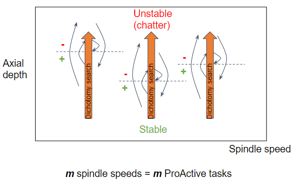Figure 2: 1st parallel version of the stability lobes research

As a first parallel version, we distribute the dichotomy stability lobes research over spindle speeds. Technically, we box the dichotomy stability lobes research in a dedicated function, we keep the spindle speeds iteration to build the input parameter list, and we call PAsolve on both, the dichotomy stability lobes research and the input parameter list, to trigger in parallel as many researches as spindle speeds.

Figure 3: Scalability tests of the 1st parallel version. Parameters are voluntarily not expose (Matlab)

All Matlab scalability tests were performed on a dual processor machine with 32Go RAM running on windows server 2008 R2 SP1. Each processor is a X5650 with 12 cores @2.67Ghz. As the graph depicts, exploiting more than 10 cores is not sufficient to break the 400s floor. By observing the task execution time range, this latter increase with the number of nodes (in minutes, from 1’21-2’25 to 2’40-3’57). Indeed, when running a high number of nodes, and by this way, executing many compute intensive tasks on the same machine, the running jvms and matlab computations overload all the CPU cores and saturate the two processors (>80%), degrading the task durations. Such scalability tests could benefit of a cloud infrastructure to reduce the CPU usage.

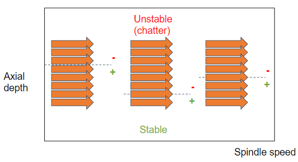Figure 4: Parallel stability lobes research with 2 levels of parallelism

In the second version, we introduce a second level of parallelism by breaking the dichotomy search into parallel stability searches over a range of cut depths (2nd level of parallelism). Technically, the input parameters list of the first parallel version is extended to consider all combinations of spindle speeds with starting cut depths.

Figure 5: Scalability tests of the 2nd parallel version. Parameters are voluntarily not exposed (Matlab)

In comparison of the first parallel version results, we observe with this second strategy that, triggering several non compute intensive tasks on more than 10 nodes, does not saturate the CPU, since it linearly decreases up to 20 cores. However, this strategy involves several ProActive tasks executions. If we keep the same spindle speeds number used for tests illustrated in Figure 2, this will trigger 800 ProActive tasks, saturating a lot our single CPU (tasks initialization and execution). Moving to scilab will afford to exploit a distributed system for our scalability tests, without the extra cost of Matlab licences.

The main drawback of Matlab is the licence cost, and since our technology requires a Matlab installation per node, the overall cost increases with the number of nodes. To break this financial constraint, we decided to rely on Scilab. For Scilab scalability tests, we used 4 m4.xlarge Amazon EC2 instances, each instance including 4 vCPU, 16Go RAM, allocated on a Intel Xeon 2,3 GHz E5-2686 v4 (Broadwell) or on a Intel Xeon 2,4 GHz E5-2676 v3 (Haswell).

Figure 6: Parallel stability lobes research following the 3rd strategy

Figure 7: Scalability tests of the 3rd parallel version. Parameters are voluntarily not exposed (Scilab)

We proposed a 3rd parallel version, which is a major update of the 2nd one. To reduce the overhead related to ProActive task initialization in case of several simulations, rather than triggering as many ProActive tasks as the total number of stabilities to estimate (2nd parallel version), we decided to only trigger as many tasks as nodes, each task having in charge a subset of the total number of the stability estimations (Figure 6).

The main advantage of the 3rd strategy is to propose a fully scalable parallel version, by breaking the bottleneck of the sequential dichotomy research. But computational resources must be high enough to reach equivalent performances to the 1st version. Indeed, by setting the same precision for all strategy (0.5/1000mm), the 1st version takes ~300s with 3 ProActive nodes against +500s for the 2 others using +10 ProActive nodes. The latest strategy seems to benefit of the ProActive tasks number reduction, and takes ~540s against ~612s for the 2nd strategy, over 12 nodes. Moreover, this latter is almost fully scalable as Figure 7 depicts.

Thanks to the scilab connector, the stability lobes research can benefit of a HPC infrastructure without the extra cost of the Matlab licence.

Figure 8: Speedup factors of the Figure 7 results